Elasticity Experiment: Application of Hooke's Law

• Nguyen Manh Tri

Investigation of elasticity

Introduction

1. General statement

Any string that able to stretch and come back its original length can be considered as a spring. Each spring has constant of elasticity (stiffness) that depends on its material. A simple spring generally is made from metal.

2. Background

Elastic forces of the springs appear at the ends of the springs and material effect on the contact or association with it as it is deformed (Elert, 1998). The direction of elastic force counters the direction of the external force causing deformation. Specifically, when stretched, the elastic force of the spring towards the axis of the spring on the inside; even when compressed, the elastic force of the spring axis oriented outwards.

The most popular law of elasticity is Hooke’s law. When a force is applied to an elastic object, the object will be stretched. A change in length ∆l is formed. In the elastic limit, the magnitude of the elastic force of the spring is proportional to the deformation of the spring. Hooke’s law can be expressed as

= k ()

where k is a constant value which shows the stiffness of the object (Belen’kiÄ­, Salaev and SuleÄ­manov, 1988). The k value has unit of newton per meter.

A spring of length l₁ is hung up by a bracket as shown in figure 1. If a mass is applied to the other end the spring, the spring will be stretched, resilient until all the energy is gone and form a new length l₂. Then the system is balanced, the applied force, the weight of the mass, must equal the restoring force

Mg = k(l₂ – l₁) = k∆l

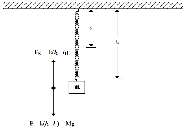
Figure 1

Mathematically, Mg = k can be written as

∆l = [1.0]

Equation [1.0] also can be performed as a linear equation (Treloar and Dunn, 1974)

y = mx

where y is ∆l and x is M.

Then if we hang more and more weights for the spring and measure the length ∆l for each, the gradient of the graph is (Bbc.co.uk, 2014). Consequently, we can find the constant value k by calculating the gradient.

For rubber or steel wire rope elastic force only when external forces are stretched. In this case the elastic force is called tension. Tension set point and direction like elastic force of the spring. For the contact surface is deformed when pressed against each other, with the elastic force perpendicular to the contact surface.

3. Aims

To determine the constant of elasticity of several different springs

To find out the elastic limit.

4. Hypothesis

There are number of factors which affect the springs’ constant. One of these factors is the types of material, which makes the stiffness of springs different. Hooke’s law is accurate with simple objects such as springs. With material such as rubber or plastics, the dependence between the elastic forces in the deformation could more complicate (Belen’kiÄ­, Salaev and SuleÄ­manov, 1988).

In essence, the elastic interaction forces between molecules or atoms, i.e. the electromagnetic force between electrons and protons inside the elastic material.

When the large deformation to a certain value, the elastic force does not appear again, and this value is called the elastic limit, if you exceed the time limit elastic deformation material will not be able to return original shape after impact not deform more.

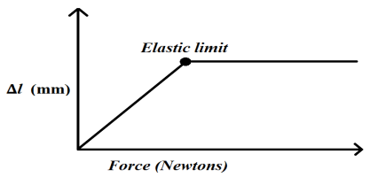
Figure 2: Elastic limit

Method and Materials

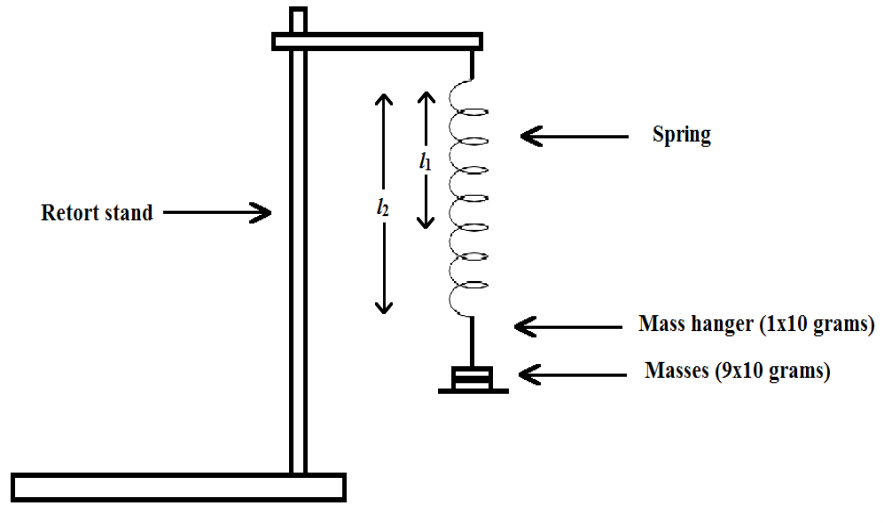
Figure 3: Experimental set-up

1. Method

1. The experiment was set up as shown in figure 3.
2. The retort stand was placed firmly on the table.
3. A spring was attached to the retort stand.
4. The length of the spring (l₁₎ in rest state was measured (using ruler) and recorded.
5. The mass hanger (10 grams) was hung up the other end of the spring.
6. New length of the spring (after applied the mass hanger) was measured (using ruler) and recorded. The change of length of the spring was calculated and recorded. One set of data was obtained afterwards.
7. A weight was placed on the mass hanger.
8. New length of the spring (after applied the weight) was measured (using ruler) and recorded. The change of length of the spring was calculated and recorded. Another set of data was obtained afterwards.
9. Another weight was placed (20 grams total) and step 8 was then repeated.
10. Step 9 was repeated until no weight left. 8 other sets of data were obtained afterwards.
11. Steps 3 to 10 were repeated for the new springs (the remaining 2 springs). Finally, 30 sets of data were obtained (10 sets each spring).

Results

Table 1: First spring results

l₁ for the first spring = 13 mm

Table 2: Second spring results

l₁ for the first spring = 20 mm

Table 3: Third spring results

l₁ for the first spring = 20 mm

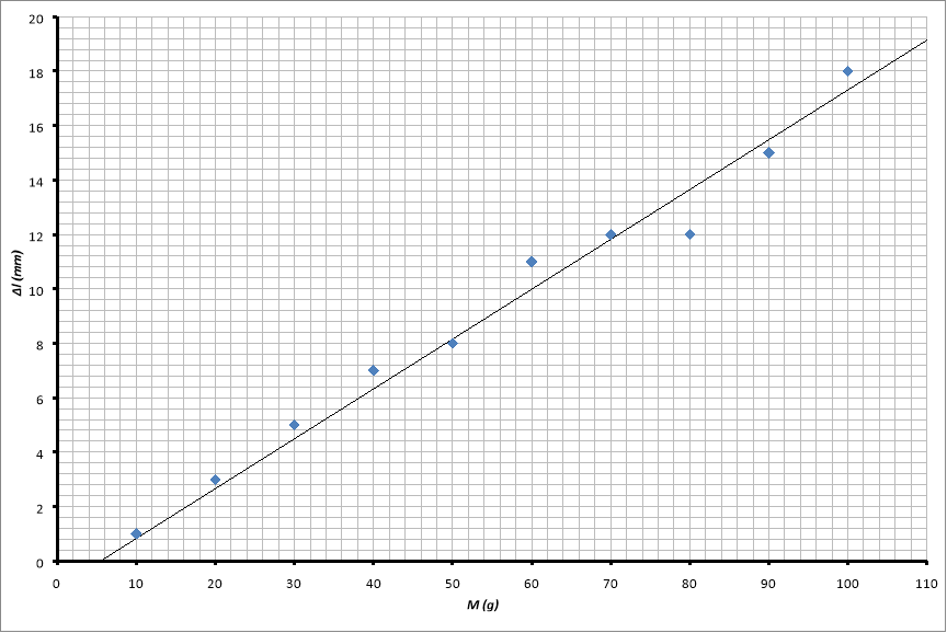
Figure 4: Change of length against mass for the first spring

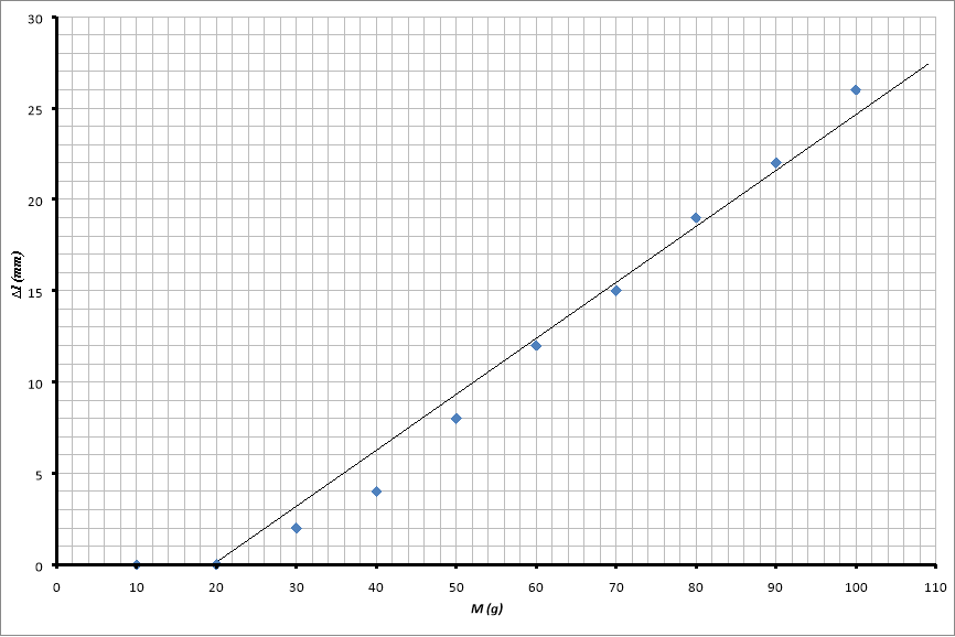
Figure 5: Change of length against mass for the second spring

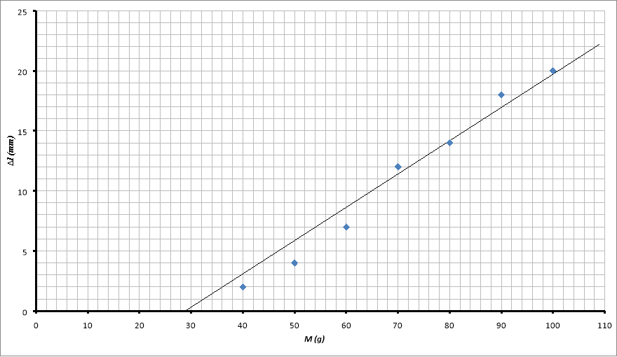
Figure 6: Change of length against mass for the third spring

As shown in figure 4, 5, and 6 three straight lines are formed and show a trend that the weight increases with increasing ∆l.

Discussion

1. Calculation – Results from part 1 experiment

From figure 4,

y = 0.1834x – 1

therefore,

gradient (m₁) = 0.1834 mm/g

From figure 5,

y = 0.3062x – 6

therefore,

gradient (m₂) = 0.3062 mm/g

From figure 6,

y = 0.2774x – 8

therefore,

gradient (m₃) = 0.2774 mm/g

Since the spring constants are measured by

gradient (m) =

therefore,

k =

We also have g = 9.81 (ms^-2),

k₁ = = = 53.50 mmgs^-2

k₂ = = = 32.04 mmgs^-2

k₃ = = = 35.36 mmgs^-2

2. Results analysis

Because of above factors, some points such as (10; 0) from figure 5 and (10; 0), (20; 0) from figure 6 are not involved in the trend line. The smallest share of the ruler is 1mm so it is unable to distinguish the ∆l between 0 gram and 10, 20 grams. Parallax error also is a cause of these strange points. Because of the very first ∆l are too small, wrong angles between eyes and ruler may cause the errors of these points.

Y-intercepts for 3 springs are -1, -6 and -8 respectively. The y-intercept -1 is a very small value and is able to show the accuracy of the experiment. The others two are much bigger because of different constant k values of springs (53.50, 32.04 and 35.36 respectively). For the first spring, which has k value are 53.50, it is much easier to distinguish different ∆l values for the first weights. Consequently, there is no strange point is recorded for this spring, all the points involves in the trend line. For the last two springs, k values are almost half of the first one and it hard to distinguish ∆l values for the first weights. This is the reason why strange points are recorded and do not involve in the trend lines. Consequently, the trend lines of these springs tend to go far away the origins when pass the y-axis.

3. Errors analysis and other factors affecting the experiment

1. Parallax error

Parallax error is the most popular error in physics (Aphysicsteacher.blogspot.co.uk, 2009). Because this experiment contain many small values (smaller than mm), so parallax error may cause many wrong data and strange points. The concept of parallax error is related to the term parallax. For instance, in figure 7, different positions of eyes result in 3 values for the measurement (two of them are wrong values).Soparallax is the change in the apparent position of an object when the position of the observer changes.

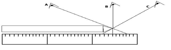
Figure 7: Example for parallax error

Consequently, the accuracy of the measurement depends on the angle between eyes and ruler. Because of this error, ∆l values are slightly greater or smaller and results in slightly change of k values. To minimize this error, a pointer can be used to help read the scale on the ruler and the scale had to be viewed at eye level (Cyberphysics.co.uk, 2014).

2. Temperature

Materials’ thermal expansion coefficient α and stiffness are connected. This connection is mathematically formulated as α = where the γ_G is a constant value (0.4 < γ_G < 4), ρ is the density.

α is a constant value so if temperature is increased, density increases and stiffness increases; if temperature decreased, density decreases and stiffness decreases.

3. Accuracy of ruler

The smallest share of plastic ruler is 1mm. As mentioned above, there are many small values so it is necessary to consider the error percentage caused by accuracy of ruler.

4. Improvement

To minimize parallax error, a pointer can be used to help read the scale on the ruler and the scale had to be viewed at eye level (Cyberphysics.co.uk, 2014).

To minimize temperature error, the air temperature should be held on standard (room temperature – 298K).

To minimize accuracy of ruler error, an instrument which has small length accurately should be used (Mohindroo, 2006). The accuracy of the result can be greatly improved.

Conclusion

The constant of elasticity of 3 springs are 53.50, 32.04 and 35.36 respectively by calculating as mentioned above. Summarizing the three points, this experiment has met the objectives stated in the introduction. Knowledge about elasticity and constant of elasticity has learnt through this study.

It is unable to find out the elastic limits because if keep adding weights until the springs can stretch more, the springs will be damaged and will not be able to come back its original shapes (Sadd, 2005).

There are some factors are mentioned above, which are affect the results of this experiment. These factors do not change the results significantly (strange points were recorded only for the very first weights).

Reference