Movement in an Idealized Dam-break Configuration
| ✅ Paper Type: Free Essay | ✅ Subject: Engineering |
| ✅ Wordcount: 1588 words | ✅ Published: 31 Aug 2017 |
For doing the research of the fluid dynamics with the open channel flow, to derive and understanding different waves equations in partial differential approximation with conservation form such as the explicit centered convection approximation and the explicit upwind convection approximation in different condition. Trying to substitutive the values into the equations to derive the appropriate method base on the finite- volume method in the fluid dynamics and using the software to calculate the flux and the stability which will depend on the direction of the wave and must be under the distance travel must not exceed the step way condition.
The aim is staring to go through the details of the equations, get the brand new Flux functions which called ‘lax Wendorff burgers equation’ scheme and Dam break scheme, based on those approximation to estimate the wave direction, wave speed, height, density and momentum in the certain and instant time for the water wave and at different conditions property and combinations. Putting the values to get the approximate results with those two methods and compare with each other. Plot the appropriate graphs.
Abstract
The purpose of this study is to model the flow movement in an idealized dam-break configuration. One-dimensional motion of a shallow flow over a rigid inclined bed is considered. The resulting shallow water equations are solved by finite volumes using the Lax-Wendroff schemes. At first, the one-dimensional model is considered in the development process. With conservative finite volume method, splitting is applied to manage the combination of hyperbolic term and source term of the shallow water equation and then to promote 1D. The simulations are validated by the comparison with flume experiments. Unsteady dam-break flow movement is found to be reasonably well captured by the model. The proposed concept could be further developed to the numerical calculation of non-Newtonian fluid or multilayers fluid flow.
All the calculations, data and graphs represent are all through MATLAB programming with an individual code and all the units and symbols were labeled in the code.
A. Units and constant for the approximations
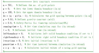
Equations &Theory
- Partial Differentials
Partial differential equations are complicated method to solve as they contain more than one variable and instead are used to
Describe problems involving the parameters in use which can be solved using the variation of schemes. They describe the certain rate of change of variables which are related to each other, in this project, the first convection are the wave equation in conservation form which are to approximate the velocity of the flow in different directions and the flux approximation with changing time. Two different methods are considered which are the explicit upwind convection approximation and explicit centered convection approximation respectively.
When dt = 0 and dx = 0,

- Discretization Schemes
Explicit centered convection approximation and explicit upwind convection approximation, these methods include finite volume method which approximating the variables around discrete nodes with dissected into too many small elements that are approximated.
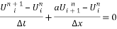
- Finite-Difference Approximation
Finite-difference approximations are one of the most derivative methods for solving differential equations. The system can approximate the solution with the necessary boundary and initial conditions imposed, providing an accurate solution for the previous unfathomable equation. They are of particular use in aerodynamics as their time and space dependent nature lends itself to computing shock wave propagation or other energy transfer flows.
Their approach uses discretization to approximate the differential, by applying a finite grid, of points at which the variables are estimated, with the process continuing as the local points govern their approximation values from the neighboring nodes. Iterative approximation in this manner produces an obvious error, known as the ‘discretization or truncation error’, diverging from the true value. The key to the principle is, like anything, minimizing this error in the system. Monitoring this error then is something of paramount importance and through the implementation of the ‘Taylor Series’.
In addition, there are three critical properties that any approximation of a partial differential should maintain, which are consistency, stability and convergence.
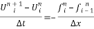
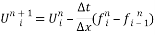
- Forward-Time, Backward-Space Scheme
The form of approximation method is a ‘backward’, explicit, hyperbolic system which means that at the next set of results are only calculated from the nodes immediately behind them geometrically, in relation to their pervious counterparts, for examples,
When dt = 0 and dx = 0,
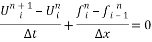
This also gives the system an inherent advantage as this encourages convergence, through the fact that the approximation method has a “domain of dependence’ which are include the initial data, shared by the partial differential at t = 0, only apply on the first set of data.
Also, further information gathered from the equation itself shows is a first order method and most suitable to simple differential approximations.
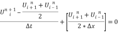
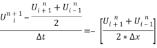
- Lax Scheme
This kind of approximations are most likely the previous is explicit hyperbolic in nature, however, it is a scheme which to demonstrated that all the velocity of the water flow  terms are either side of
  and is first order accurate for u, and also approximate the accuracy for x.
When dt = 0 and dx = 0,
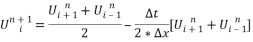
Moreover, the stability of the method has to be considered as the Courant-Friedrichs-Lewy (CFL) condition is a necessary condition for convergence while solving certain partial differential equations usually hyperbolic numerically by the method of finite differences. It arises in the numerical analysis of explicit time integration schemes, when these are used for the numerical solution. As a consequence, the time step must be less than a certain time in many explicit time-marching computer simulations, otherwise the simulation will produce incorrect results.

- Lax-Wendroff Scheme
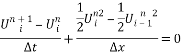
This scheme is a common numerical method for the solution of hyperbolic partial differential equations like the previous schemes which are based on the finite differences to accurate for both space and time apparently. There are two different cases are going to consider and approximate which are the 1st for the linear case, while
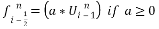
 , where a is a constant which to define the direction of the flow and u is the wave speed, when
 , the flow is to the right, and to the left when a is negative. As two different approximations have considered, for the centered method
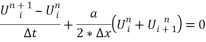

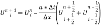
For the upwind method
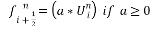
Or 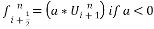
Or 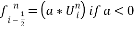
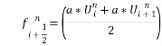
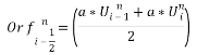
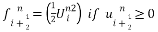
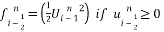
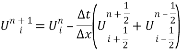
And for the Lax-Wendroff in first-order
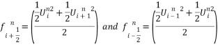
Predictor,
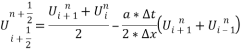
Corrector,
For the 2nd case, 

Centered method
For the upwind method
 Or
Or 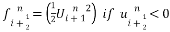
 Or
Or 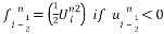
And for the Lax-Wendroff in first-order
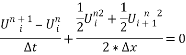
Predictor,
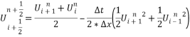
Corrector,
Calculate for the half grid points and time steps approximation as different predictors first and then recalculate the scheme by the value of half grid points and time steps into same Corrector which putting a two steps approximation rather than a single step to make it more accurate. This is a feature unique for the Lax-Wendroff method. Also, the stability of CFL condition is the same as the previous scheme.
- Taylor Series
The Taylor series is a form of evaluating and representing partial differentials, as an infinite sum of its terms at a single point, in form of series expansion. The use of the series has many applications in engineering, with its main being the approximation of functions through the expansion to the necessary number of terms. Through collating the appropriate number of terms and then ‘truncating’ the series a valid approximation of the function can be made. The act of truncating the series generates an error, although as the expansion continues the effect of each term dwindles, a characteristic that allows the truncation after a certain term number. The truncation error can also be computed and gives an indication as to the validity and performance of the initial approximation made using the series expansion.
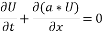
B. Dam break schme
The simplest situations will first be considered, of mass, momentum and energy conservation laws in primitive form, so stripped of all energy-diffusing terms, such as bed slope , resistance, change of section.
Governing Equations

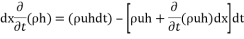
The mass entering t element in time dt is

While the amount leaving is
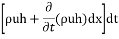
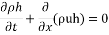
For the mass
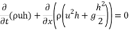
For the momentum
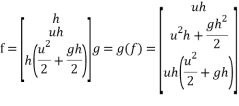
For the simplest case, 
X1
Figures and Tables
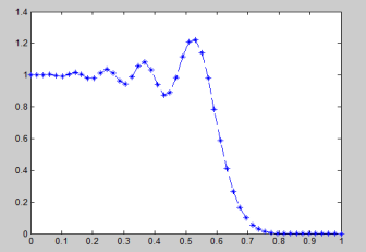
Figure 1
Figure 1 shows the relationship of the velocity against the postion of the flow in linear first-order which (f = a*u) , where a is 1, Lax-Wendroff is used for approximation, and it shows a steady flow with a certain time and positions with the input data, there are 50 nodes in total and the grid spacing are 400 as the detla time was 0.0015s, so the grid spacing should have to take a really large value to maintain the CFL.
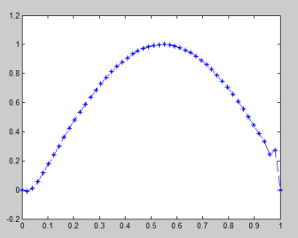
Figure 2
Figure 2 shows the relationship of the velocity against the postion of the flow in non-linear first-order which (f = u2/2), Lax-Wendroff is used for approximation, and it shows a steady flow with a certain time and positions with the input data, there are 50 nodes in total and the grid spacing are 30 as the detla time was 0.0015s, the grid spacing take a really smaller value to maintain the CFL.
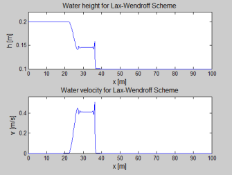
Figure 3
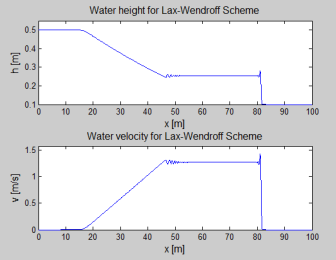
Figure 4
Figure 3 & Figure 4 shows the relationship between the height against the spacing and the momentum against the spacing respectively, dam break scheme is used with base on a Lax-Wendroff approximation and for Figure 3, the running time is 10 seconds which is shorter then Figure 4 and the depth of the dam wall sets as 0.2m and break at 30m while Figure 4 sets as 0.5m depth and break at 50m. As the results show, the longer running time it takes, the stability and convergence of the approximation comes out. Also, both of the results withdraw the boundary which take an error while plot graph. So, a function for boundary condition has to be considered as well.
References
- Guymon, Gary L. “A Finite Element Solution Of The One-Dimensional Diffusion-Convection Equation”. Water Resources Research 6.1 (1970): 204-210. Web.
Cite This Work
To export a reference to this article please select a referencing stye below:
Related Services
View all


DMCA / Removal Request
If you are the original writer of this essay and no longer wish to have your work published on UKEssays.com then please click the following link to email our support team:
Request essay removal