MaxEnt vs K-Nearest Neighbour
| ✓ Paper Type: Free Assignment | ✓ Study Level: University / Undergraduate |
| ✓ Wordcount: 2845 words | ✓ Published: 13 Oct 2021 |
Exercise 0: What are the new correctly classified instances, and the new confusion matrix? Briefly explain the reason behind your observation.
Logistic Regression (Max Entropy)

Figure 1 – Weka Output – Correctly Classified Instances (Logistic Regression)
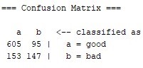
Figure 2 – Weka Output – Confusion Matrix (Logistic Regression)
Using logistic regression, 752 of instances were correctly classified out of the 1000 instances in this dataset (75.2%). In terms of the resultant confusion matrix shown in figure 2, the number of correctly classified instances can be calculated through the addition of the true positive (position: (0,0)) and the true negative (position: (1,1)) values ((605+147)/1000=75.2%). As seen in figure 2, the number of correctly classified instances of the “good” class (true positive), is 605. In the context of the data provided (credit-g.arff), it is implied that 605 borrowers were able to repay their loan. In contrast, the number of correctly classified instances of the “bad” class (true negative), is 147; for which, it is implied that 147 borrowers were not able to repay their loan.
In terms of the classification of the data, the logistic regression model classifies the datapoints given a linear boundary for which, the distance between the datapoints and the boundary is used for classification between the “good” and “bad” classes.
K-Nearest Neighbours (KNN k=1)

Figure 3 – Weka Output (KNN Classifier k=1) – Correctly Classified instances
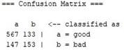
Figure 4- Weka Output – Confusion Matrix – (KNN Classifier k=1)
Using the K-Nearest Neighbours model where k=1, 720 instances were correctly classified out of the 1000 instances in this dataset (72%). Lower than the logistic regression model seen in figure 1, which is the result of using a different approach to classification, whereby the distance between one datapoint and a k number of its closest datapoints (in this case one neighbour) is evaluated in order to classify datapoints into decision regions (in this case, the “good” and “bad” decision regions).
Using the low k value of 1, the number of correctly classified instances is shown to yield a lower value to that of the logistic regression model. This may be due to the fact that when only one neighbour is being evaluated, the model will start to fit the data too well, resulting in overfitting of the dataset and ultimately, a lower number of correctly classified instances.
The resultant confusion matrix shown in figure 4 denotes the true positive (correctly classified “good”) number of instances to be 567 and the true negative (correctly classified as “bad”) number of instances to be 153 ((567+153)/1000=72%) however the number of incorrectly classes is shown to be higher with a false positive (incorrectly classified as “bad”) value of 133 and a false negative (incorrectly classified as “good”) value of 147 ((133+147)/1000=28%). This is due to the fact that using one neighbour as an evaluation reference for classification makes the decision-making process difficult when trying to find out where a majority of the datapoints in the sample lie in terms of the decision boundary. K-Nearest Neighbours (KNN k=4)

Figure 5 – Weka Output – Correctly Classified instances (KNN Classifier k=4)
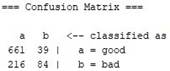
Figure 6 – Weka Output – Confusion Matrix (KNN Classifier k=4)
Using a higher k value of 4 in the K-Nearest Neighbours classification algorithm, the number of correctly classified instances of the data yields an improved to 745 instances out of the 1000 instances in the dataset (74.5%). The resultant confusion matrix shown in figure 6 shows a higher true positive (correctly classified as “good”) of 661 and a lower true negative value of 84. The difference in the values between KNN where k=1 and k=4, is due to the fact that using a higher k value allows for more comparisons between one datapoint and an increased number of nearest neighbours, thus decreasing the chances of the model fitting the data too closely (chances of overfitting decreases). Although the chances of overfitting have decreased, there is still a chance for the model to be unable to capture the underlying trend in the data to use for classification (underfitting).
K-Nearest Neighbours (KNN k=999)

Figure 7 – Weka Output – Correctly Classified instances (KNN Classifier k=999)
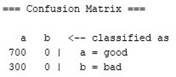
Figure 8 – Weka Output – Confusion Matrix (KNN Classifier k=4)
Using a very high k value of 999 for K-Nearest Neighbours Classification yields the lowest number of correctly classified instances of 700 out of the 1000 instances in the dataset. This is because each datapoint being evaluated has been compared to every other datapoint in the dataset excluding itself. This methodology has given leeway for major underfitting to take place as every datapoint was predicted and actually classified as “good”, thus, resulting in no “bad” classifications of the datapoints. This is proven in the confusion matrix shown in figure 8 where the “good” number of correctly classified instances (true positive) is 700 and the number of incorrectly classified instances of “good” datapoints (false negative) is 300.
OBSERVATIONS
The point of classification is to be able to correctly classify as many instances of the dataset into the right groups with minimal wrong predictions. In this case, using the MaxEnt classifier works the best.
The “sweet spot” between the values of k is required because past k = 4, true positive decreases and as it gets to 999 or samplesize-1, underfitting takes place. Overfitting occurs at k=1
Out of all of the values of k for the K-Nearest Neighbour classifier, the k-value of 4 holds the best and most accurate number of classified instances. As the value ok k increases past 4, the number of correctly classified instances reduces (in the case of k=5, the no of correct instances is 742 or 74.2%)
Observation and conclusion for correctly classified instances: logistic regression holds the highest percentage of correctly classified instances.
Exercise 1: Try (by varying the values of weights in the code), and describe the effect of the following actions on the classifier (with a brief explanation)
- changing the first weight dimension, i.e., w0 ?
- changing the second two parameters, w1 , w2 ?
- negating all the weights?
- scaling the second two weights up or down (e.g. dividing or multiplying both w1 and w2 by 10)?
Changing the first weight dimension (w0):
Keeping the initial values of w1 and w2 the same, by changing the first weight dimension (w0), the position of the boundary shifts to the left or the right. When the value of w0 is positive, the boundary shifts to the right; in contrast, when the value of w0 is negative, the boundary shifts to the left. This is because in the logistic function, as the value of w0 increases, the resultant exponent is effectively penalised as it yields a lesser value. This is shown visually as when the boundary shifts to the right, the colour red becomes more prevalent as Pr(label=1) yields a higher value (which shows a bias towards label 1). When the boundary shifts to the left, the colour blue is more prevalent as Pr(label=1) yields a lower value (which effectively penalises the logistic function).
Changing the other two parameters (w1,w2):
By keeping w0 and w2 constant, changing the value of w1 from -5 to -25 (as a negative weight) shows that the width of the boundary shrinks and it is implied that w1 changes the overall width of the boundary. This is shown visually as when the boundary shrinks (as the value of w1 increases), the resultant colours show less of a gradient and more of a solid yellow line down the colour spectrum with minimal gradient. As a positive weight, the boundary is effectively inverted, showing the colours in the spectrum at opposite sides than the original.
By keeping w0 and w1 constant, changing the value of w2 will change the slope of the boundary line. As a positive weight, the boundary slope is shown visually as an upwards diagonal slope; As a negative weight, the boundary slope is shown visually as a downwards slope.
Negating all the weights:
Assuming that negation could be achieved by setting all of the weights to a value of 0, the entire colour spectrum develops into blue which covers all datapoints, which effectively means that the dataset is classified as 0. Assuming that negation could also be achieved by inverting the original weight from (0, -5, 0) to (0, 5, 0), as highlighted earlier, the boundary becomes inverted, showing the colours in the spectrum at opposite sides than the original.
Scaling the second two weights up or down:
Scaling the second two weights up by 20 from the original, making (0, -5, 0) become (0, -100, 0) will affect the boundary line by making it thin and narrow. When scaling w1 as a positive weight (making (0, -5, 0) become (0, 100, 0) by scaling by -20) seems to have the same effect in terms of the boundary line width becoming narrow.
Scaling the second two weights up by 20 when w2 is positive or negative 1, making (0, -5, 1) and (0, 5, -1) become (0, -100, 20) and (0, -100, -20) creates a thin boundary which is sloped upwards when w2 is 20 and creates a downward slope when w2 is -20.
However, by scaling the second two weights (using the original weights (0, -5, 0)) down by a value of 1/5 (0.2) making the resultant weights (0, -1, 0), the boundary line becomes very wide which implies that the thickness of the boundary line increases as the value of the weight is greater or less than but not equal to 0. Scaling the original weights down by a scale factor of -0.2 making the weights (0, 1, 0) inverts the boundary line however it stays wide in width.
By scaling both w1 and w2 upwards or downwards, the boundary will change in width and will gain an upwards or downwards slope when positive or negative respectively.
Exercise 1: (a) How many times did your loop execute? (b) Report your classifier weights that first get you at least 75% train accuracy.
a) The loop executes 8000 times (achieved by a simple count incrementor)
b) The classifier weights which first yield at least 75% train accuracy are: [-0.579 1.000 0.789]
Exercise 2: (a) Notice that we used the negative of the gradient to update the weights. Explain why. (b) Given the gradient at the new point, determine (in terms of “increase” or “decrease”, no need to give values), what we should do to each of w0 , w1 and w2 to further improve the loss function.
a) Using a negative gradient to update the weights (also known as gradient descent) allows the minimisation of the cost function due to the fact that identifying a model with minimum error can prove to be costly. This is an iterative process which allows for a lower loss function value to be reached whilst updating the coefficients to step in the direction of the steepest descent.
b) The gradient at the new point shows that the weight w0 increased whilst weights w1 and w2 have decreased. Another observation for the gradient at the new point is that the loss function value has decreased while the train accuracy has increased. To further improve the loss function value, it is imperative that the gradient descent process moves in the general direction of the steepest descent (the negative gradient) so that the loss function can be reduced to a smaller value.
Exercise 3: Suppose we wanted to turn this step into an algorithm that sequentially takes such steps to get to the optimal solution. What is the effect of “step-size”? Your answer should be in terms of the trade-offs, i.e., pros and cos, in choosing a big value for step-size versus a small value for step-size.
Step size is essential when attempting to get as close to the optimal solution as possible. This is due to the fact that using a big step size can lead to “overshooting” and a small step size will converge on the optimal solution slowly. Below are the pros and cons of the step size used:
A big value step size may seem like a good method to finding the optimal solution as it provides fast results. However, although this is said, when the step size is too large, there is a high chance that “overshooting” (or “overstepping”) can take place where the algorithm goes past the minimum point (the objective being to reach the global minima) which will in-turn diverge from the optimal solution.
A small value step size is less likely to “overshoot” the minimum point as it iterates using miniscule steps (in comparison to big value step sizes) to find a more accurate solution however, considering that the algorithm is iterative and is likely to span many iterations, the time in which it takes to iterate through small step sizes will be time consuming and computationally more expensive due to more iterations being completed during computations (as opposed to big step sizes).
Overall, considering both types of step size, a suggested method is to either implement a calculation which allows the next step size to be computed at each iteration using a varying number of step size values in order to guide the stepping process when finding the optimal solution. This will allow the model to recognise the direction in which to step and identify the ideal distance to move in that particular direction. Another method is to
Exercise 4: Answer this question either by doing a bit of research, or looking at some source codes, or thinking about them yourself:
(a) Argue why choosing a constant value for step_size, whether big or small, is not a good idea. A better idea should be to change the value of step-size along the way. Explain whether the general rule should be to decrease the value of step-size or increase it.
(b) Come up with the stopping rule of the gradient descent algorithm which was described from a high level at the start of this section. That is, come up with (at least two) rules that if either one of them is reached, the algorithm should stop and report the results. [0.5 + 0.5 = 1 mark]
a) It is not ideal to keep a constant value for the step size regardless of the size when trying to find the optimal solution. This is based on the drawbacks of both types of step sizes whereby overstepping the minimum point may occur or using a model which finds the optimal solution time consuming and computationally expensive manner. As suggested previously, a better idea for an implementation for step size is to vary the value of the step size by changing it at each iteration. Based on research, it is better to start off with a relatively large step size and as each iteration passes, calculate a smaller step size to allow for the model to recognise the optimal distance to the next step and the direction in which it would need to take in order to reach the minimum point (the optimal solution). This would reduce the chances of the model overstepping the minimum point and coincidentally allows for a fast but computationally cheaper solution when trying to find the minimum point (optimal solution). This will also allow the model to learn the general location of the minimum point.
b) In terms of a stopping rule for the gradient descent algorithm, the goal is to minimise the drawbacks of utilising certain step sizes (both big and small). In order to make the algorithm computationally cheaper, a maximum number of iterations can be defined where the model will stop at a given number of iteration and will output the results. This goal can also be achieved using a stopping criterion for the time in which computations take place so that resources are not completely exploited. Another stopping criterion which could be applied is to use smaller steps at a set limit given by a general threshold and then stop. This is so that once the threshold is reached, the model can use smaller steps when in the general location of a minimum point and return the results which, will in-turn reduce the number of computations required and thus makes the algorithm computationally cheaper.
Exercise 5: Provide one advantage and one disadvantage of using exhaustive search for optimisation, especially in the context of training a model in machine learning.
One advantage of using exhaustive search for optimisation when training a model in machine learning is that the algorithm explores different combinations of the weights using a brute force approach in order to find the combination of weights which gives the lowest loss function value. Although this is said, the main drawback to this methodology is the fact that it is a brute force approach, meaning that the process can be lengthy and cannot assure that it will perform the same when test data is used. This is due to the fact that the combinations of weights will vary amongst datasets.
Exercise 6: (a) What is the best value for K ? Explain how you got to this solution. (b) Interpret the main trends in the plot. In particular, specify which parts correspond to under-fitting and which part with over-fitting.
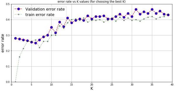
Figure 9 – Error Rate Versus K Values
a) As seen in figure 9, the best value for K would be 6. From observing the graph, it is visually the lowest error rate and by finding the value of error_test[5], it has the lowest value out of all k values (0.25).
b) The main trend which is observed from figure 9 is that as the value of k increases, the error rate increases for both the train and test errors. From K=10 onwards, both the test and train errors are visibly high, thus, underfitting is occurring. When k<5, the train errors are visibly lower than the test errors, thus overfitting is occurring.
Exercise 7: Given what you learned from this entire lab(!), provide one advantage and one disadvantage of using MaxEnt vs KNN.
MaxEnt
One advantage of MaxEnt is that it is a simple method of classification which can provide more data than most classification methods. One of the reasons for this advantage is that the MaxEnt model can express how relevant a predictor has been as seen in question 0.
One disadvantage of MaxEnt (Logistic Regression) is that it cannot be used for classification scenarios where the classes of data are not linearly separable. This means that datapoints cannot be separated into classes unless the decision boundary is linear (distinct) and where there is no distinct decision boundary, there are difficulties when classifying datapoints into classes.
KNN
One advantage of KNN is that it can be used for classification where classes are not linearly separable. This is due to the fact that KNN evaluates the distance between a datapoint and its k (value) of nearest neighbours.
One disadvantage of KNN is that the value of k needs to be defined. When choosing the best model for KNN, multiple values of k have to be evaluated by finding the “sweet spot” for the best classification model.
Cite This Work
To export a reference to this article please select a referencing stye below:
Related Services
View all


DMCA / Removal Request
If you are the original writer of this assignment and no longer wish to have your work published on UKEssays.com then please click the following link to email our support team:
Request essay removal